Economic Order Quantity: EOQ Formula + Excel Guide

If you’ve ever wondered how much and how often you should order, the EOQ formula (Economic Order Quantity or Wilson Formula) is your answer.

In this guide, I’ll break down everything you need to know about EOQ, walking you through each step with practical examples in Excel.

By the end, you’ll be ready to:

• Calculate your EOQ
• Tackle common issues related to EOQ
• Make your inventory management smoother and more efficient

Let’s dive in!

Economic Order Quantity: Definition & Meaning

The Economic Order Quantity (EOQ), also known as the Wilson formula, helps you pinpoint the ideal inventory order size.

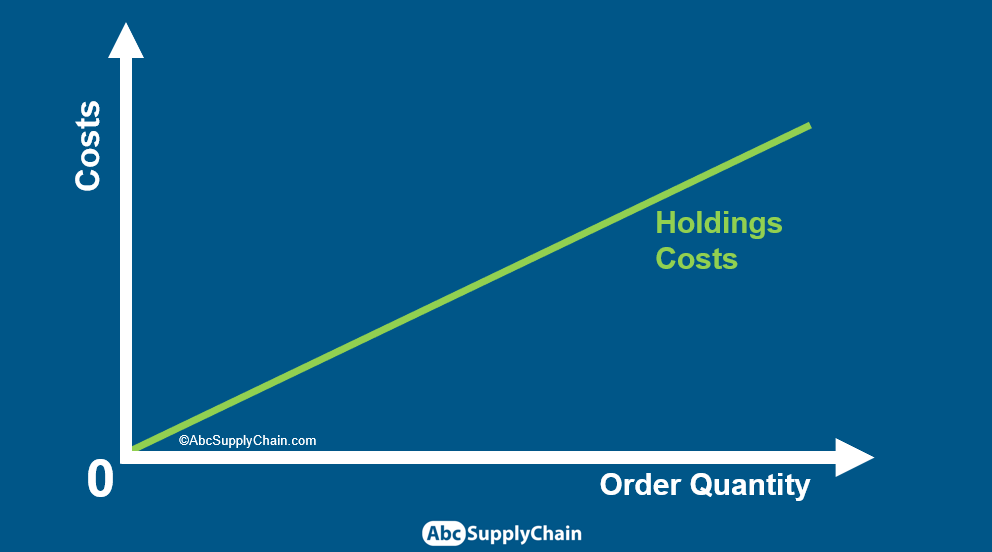
The goal is to strike a balance between two cost drivers:

These costs create two opposing curves. The Total Cost curve, the sum of Holding and Ordering Costs, reaches its minimum where the two costs are equal.

This intersection represents the EOQ, the optimal order quantity that minimizes total costs.

EOQ Formula

Instead of visualizing costs to find the balance point, going straight to the math is easier.

Here is the EOQ formula:

To calculate EOQ, you only need three numbers:

D = Demand (your forecasted consumption)
TC = Transaction Costs (cost per order)
HC = Holding Costs (cost to keep one unit in stock)

Plugging these into the EOQ formula gives you the optimal order quantity, Q—the exact amount to order to keep inventory costs at their lowest.

EOQ Calculation in Excel: Step-by-Step Guide

In this example, we’ll use Nike shoes to walk through an EOQ calculation in Excel.

1. Download the EOQ Calculator

Start by downloading our template for ease.

2. Set up your parameters

Demand

Enter your annual demand for the product. For this example, we assume a steady demand of 12,000 pairs of Nike shoes in size 43.

Holding cost

The holding Cost (HC) is the cost of keeping inventory in your warehouse, store, or factory. Many people underestimate this cost, focusing only on cash outflows and storage expenses. But there’s more involved:

• Annual Unit Storage Cost: Either as a percentage of the item value or a flat rate.
• Insurance Costs: Often a percentage of your stock value.
• Cash Costs: Interest or credit fees tied to financing the inventory.
• Theft and Inventory Shrinkage: Losses from theft or discrepancies.
• Promotion Costs: The annual promotion volume as a proportion of your total sales turnover.

In this example, we’re using a percentage of the item’s purchase price for simplicity. For accurate values, I recommend talking to your Finance Department, as they’ll have precise data on these cost factors.

The total Holding Costs for our Nike shoes are $2.85, which represents 9.5% of the purchase price.

Transaction costs

Calculating the cost of placing an order (Transaction Costs ) can be tricky because it’s more than a single expense. It includes all the fixed costs of each process involved in placing every order.

You have two common calculation methods. Let’s break it down:

• Basic Method: One approach is to take all costs from departments and people involved in order placement and divide by the total orders per year. But there’s a catch: employees usually don’t spend 100% of their time on orders alone. So this method often overestimates transaction costs.
• Recommended Method (More Accurate): Estimate the time spent on each specific process for an order. Then, multiply each by an average hourly wage.
  
  Here’s a list of typical processes (adjust this list as needed based on your operations):

Let’s say it takes 1.7 hours to complete an order. With an average $42.50 per order, this is your fixed transaction cost.

This approach gives you a clearer, more precise look at your costs and lets you make data-backed decisions on where to cut down.

Application of the EOQ Formula

Now, we can apply the formula:

D = Demand = 12,000
TC = Transaction Costs = $42.5
HC = Holding Costs = $2.85

We get an EOQ of 598 qty. As it is simpler to use round values for order management, we can round up the final result:

The annual order frequency (N) is simply the annual demand (D) divided by the quantity per order (Q). With Q set to the EOQ:

To get the frequency of orders over the year, we must divide the number of days per year by the number of orders:

Here is a summary diagram of the example:

EOQ Calculation: An Example with Lower Demand

This time, let’s consider a fancier pair of shoes with:

• Annual Demand (D) = 1,000 units (lower demand)
• Higher Holding Cost (HC) due to a higher purchase price
• Transaction Cost (TC) = unchanged from the previous example

Since demand is lower and holding costs are higher, this leads to a lower Economic Order Quantity (EOQ). In other words, more expensive, lower-demand products are ordered less frequently.

For this item, we end up placing an order every 2 months, compared to every 18 days in the first example.

This contrast highlights how demand and holding costs influence order frequency.

5 Limits of the EOQ in inventory management

The EOQ formula has some limits.

The main problem is that we consider all parameters are constant.

Limit 1: Unstable demand

EOQ assumes constant demand, but in reality, demand fluctuates due to seasonality or unpredictable peaks.

If demand isn’t steady, ordering the same quantity every 18 days, for example, can lead to overstocking during low-demand periods or stockouts during high-demand peaks.

Solution: Use a Dynamic EOQ

With a Dynamic EOQ, you calculate the EOQ with forecasted demand, tailoring order frequency to demand cycles. This keeps your inventory aligned with real demand—avoiding overstock during slow periods and stockouts when demand spikes.

Limit 2: Fluctuating Purchase Price

EOQ also assumes a fixed purchase price, but suppliers often offer quantity discounts. Sometimes, these discounts can make a larger order quantity more cost-effective than the EOQ.

Solution: Work with suppliers to map out discount tiers and see where bigger orders save you more than EOQ alone. If the discount is worth it, increase the order size.

Limit 3: Inconsistent costs

The EOQ formula assumes stable costs across transportation and storage. In practice, you can have fixed costs in a warehouse (rent, depreciation of machines) but also variable costs like workforce or electricity.

Solution: Don’t chase perfection. Focus on the costs that impact your bottom line most. Estimate them as a percentage of the purchase price to keep things simple and effective.

Limit 4: Inconsistent or unpredictable lead time

We assumed supply lead time is stable when calculating order frequency based on the EOQ. But that’s rarely true. Seasonal delays, supply chain disruptions, and holiday slowdowns can all throw off timing.

Solution: calculate your lead time uncertainty.

Limit 5: No Safety Stock

EOQ alone doesn’t cover your back against supply and demand fluctuations. You’re vulnerable to stockouts when things go off-plan, hurting your profits and customer satisfaction. That’s why EOQ is rarely used alone; it must be part of a full inventory control strategy.

Solution: Pair EOQ with other inventory controls, like safety stock and reorder points.

Bottom Line

EOQ is a solid starting point, but remember:

• Bulk discounts can justify larger orders.
• Demand and lead time aren’t always stable, so you need flexibility.
• EOQ isn’t a one-stop solution. For real-world success, integrate it with a full inventory control system.

By tackling these limitations, EOQ becomes a powerful tool rather than just a theoretical number.

The EOQ may be too simple for the complex world of the supply chain. But it’s a solid starting point. In my experience, many businesses struggle with order management basics. In that case, adding simple inventory principles can be a game-changer.

Bottom Line: Don’t wait for perfection. Start taking action today. As Jeff Bezos says:

Most decisions should probably be made somewhere around 70% of the information you wish you had. If you wait for 90%, in most cases, you’re probably slow.Jeff Bezos

EOQ: Your Action Plan

1. Download EOQ calculator here.
2. Calculate the EOQ with a few of your most important products. Once you’re comfortable, apply it progressively across your entire product portfolio.
3. Compare with Current Order Quantities: Check the EOQ results against your current quantities. This step is crucial—identify any major differences.
4. Adjust for Major Deviations: Make adjustments to align with EOQ, especially where there are significant deviations. This ensures your ordering strategy is optimized.
5. Review Production Batch Sizes, Orders, and MOQ: Evaluate your current batch sizes, order quantities, and Minimum Order Quantities (MOQ) to ensure they support your updated inventory approach.

Following these steps will give you a strong foundation for optimizing inventory.

Key takeaways from this article