Seasonality Forecasting in Excel: Predict Sales Peaks with Confidence

Seasonality forecasting is what helps you prepare for sales peaks, avoid panic, and keep your supply chain running smoothly

I’ll show you how to incorporate seasonal elements into your statistical forecasts, helping you minimize negative impacts on your inventory, and costs.

You can download the Excel Template below:

Download the Excel

Why consider seasonality in sales forecasts?

Seasonality helps allocate the right resources at the right time: inventory, money, staff, energy, communication efforts, and your time

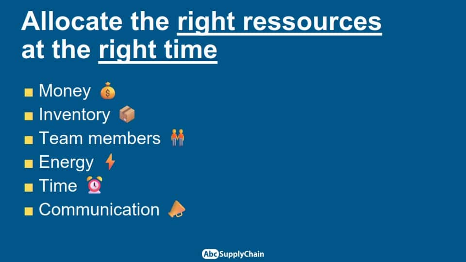
Anticipating seasonal cycle variations allows companies to allocate the right workforce, improve communication, and avoid stockouts or stressful periods caused by poor preparation. It also helps optimize stock allocation, whether on a global scale or at a very local level—in warehouses, factories, or retail stores

In this tutorial, I’ll share many practical examples to help you incorporate seasonality into your forecasts and gain both efficiency and peace of mind.

Anticipate sales peaks

This example shows a sales peak:

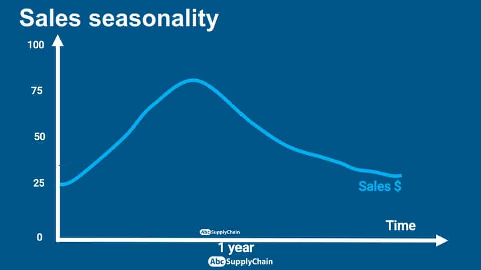
If it is poorly anticipated, without proper communication or adequately allocated resources, such as stock, staff, and logistics, it can quickly lead to stockouts, emergency situations to manage, and a great deal of stress. This is why identifying seasonal cycles and integrating them into your forecasts is so important.

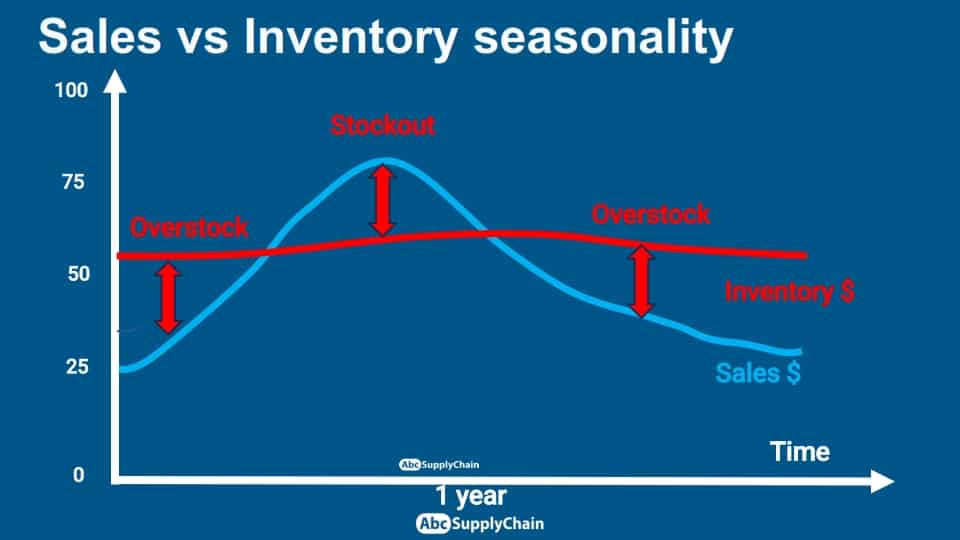
The goal is simple: identify seasonal cycles and incorporate them into your forecasts and supply chain.

This leads to better anticipation, improved organization, and, most importantly, greater peace of mind in day-to-day operations.

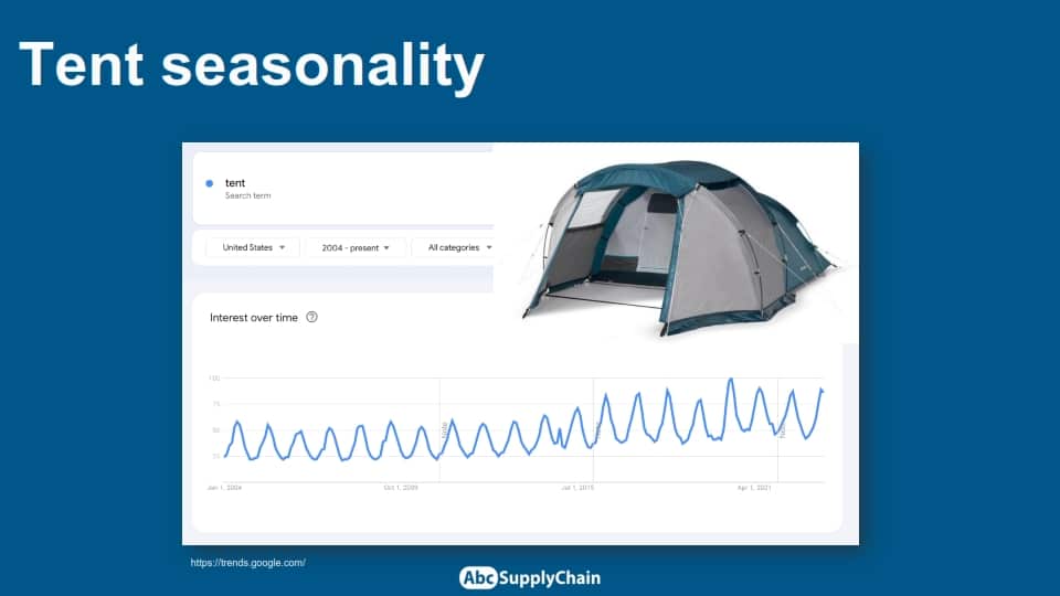
Example: Tent searches

Tent searches in the United States follow a very clear seasonal pattern: they surge in the spring, right before the holidays. Having worked for several years at Decathlon, I’m very familiar with this type of seasonality, which perfectly illustrates the importance of anticipating these peaks.

The different seasonal factors

• The Weather
  Climate has a direct impact on buying behavior. For example, tent sales rise significantly in the spring, with the return of warmer, sunnier days
• Holidays
  Time off triggers specific consumption peaks (leisure equipment, travel, food, etc.). In the United States, tent searches surge just before vacation periods.
• Recurring Events
  Major events like the World Cup peak demand for certain products (jerseys, TVs, snacks, etc.).
• Cultural Events
  Dates such as Valentine’s Day strongly influence the sales of specific products, such as diamonds, chocolates, or flowers.
• Economic Factors
  The state of the economy — both short-term and long-term — affects demand. For instance, a crisis can dampen overall consumption, while a recovery can boost certain categories.
• Planning
  Internal organization also impacts cycles: for example, if a factory is closed on Sundays, it must adjust production on the remaining days, which affects weekly output volumes. (This is a capacity-driven seasonal factor, rather than demand-driven.)

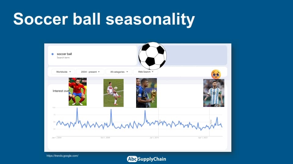
The example of the World Cup: anticipating major exceptional cycles

Some events, like the World Cup, create very important sales peaks. When I worked at Decathlon, we observed a sharp increase in football sales every four years, with one recent exception due to the pandemic, which extended the cycle to five years.
Even though these events are predictable, they still require careful anticipation to adjust stock levels and resources in advance. Failing to do so can lead to stockouts and missed opportunities.

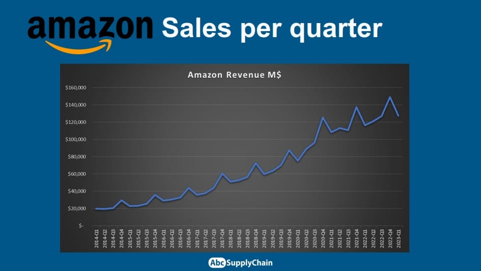
The example of Amazon: growth driven by seasonality

When analyzing Amazon’s quarterly sales, we see an overall upward trend, marked by strong seasonality.
Each fourth quarter shows a noticeable peak, largely driven by Christmas and major commercial events like Prime Day.

I explore this analysis of Amazon’s sales in more detail in my article on forecasting with ChatGPT.

This second example clearly shows that even within continuous growth, seasonal effects remain highly significant and must be factored into forecasting.

The different possible timeframes:

There are a wide variety of time cycles, ranging from one year to one second, to suit the specific needs of different business sectors.

• Year: Long-term financial forecasts.
• Month: Sales forecasts, on a shorter scale than the year.
• Week: Team planning, often with tasks defined by week.
• Day: Production planning, with daily organisation.
• Hour: Picking in the warehouse is optimized on an hourly basis.
• Minute: Tracking the performance of an energy supplier, down to the minute.
• Second: Follow-up in stock market trading, where every second can count for a lot.

• Consumption cycles can be analysed over different periods: monthly, daily and even hourly.
• Example: Energy consumption increases when it’s cold and varies throughout the day.
• There is a peak in consumption at the end of the day, followed by a fall at night and a further rise at breakfast.

Objective of seasonality in forecasting:

A good estimate of seasonality means more accurate forecasts, in other words an increase in your forecast accuracy KPI.

Ultimately, more reliable forecasts will enable you to allocate the right resources at the right time, saving you time, money, peace of mind, etc.

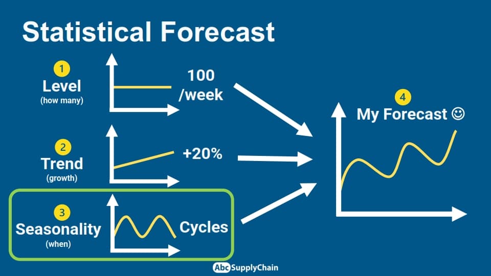
Seasonality for statistical forecasts

Seasonality is one of the 3 essential pillars of simple statistical forecasting:

1. Level
2. Trend
3. Seasonality

In this section, I’ll explain how to implement seasonality in your forecasts and show you an Excel formula for automatically detecting seasonal cycles.

I invite you to download the Excel file to practise together on two concrete examples: Amazon sales and bicycle sales.

We’ll start with quarterly seasonality and then move on to monthly analysis, with a few practical tips.

Download the Excel file

Implementing seasonality: Amazon example

In this example, we analyse Amazon’s sales using a database already explored in a previous article on forecasting with ChatGPT.

The main objective is to determine whether there is any seasonality in these sales.

Calculating seasonality by quarter

We start by examining the data through graphs, which we can create at different levels: global, by product category, or on a more detailed scale. Although some product categories don’t show regular cycles, we can see that on a global scale, Amazon’s sales follow a repeating cycle.

This clearly suggests the presence of seasonality, but we need to verify this by calculation, using the Excel formula FORECAST.ETS.SEASONALITY This function is used to analyse repetitive cycles in a time series:

• In cell I10 for this example, we enter the formula FORECAST.ETS.SEASONALITY
• We select column F, including revenues (here Table2[Revenue M$] because it is the column of a table) for the first parameter
• The second parameter is column A (Table2[ID]), which simply contains the values 1,2,3…up to the end of the table.

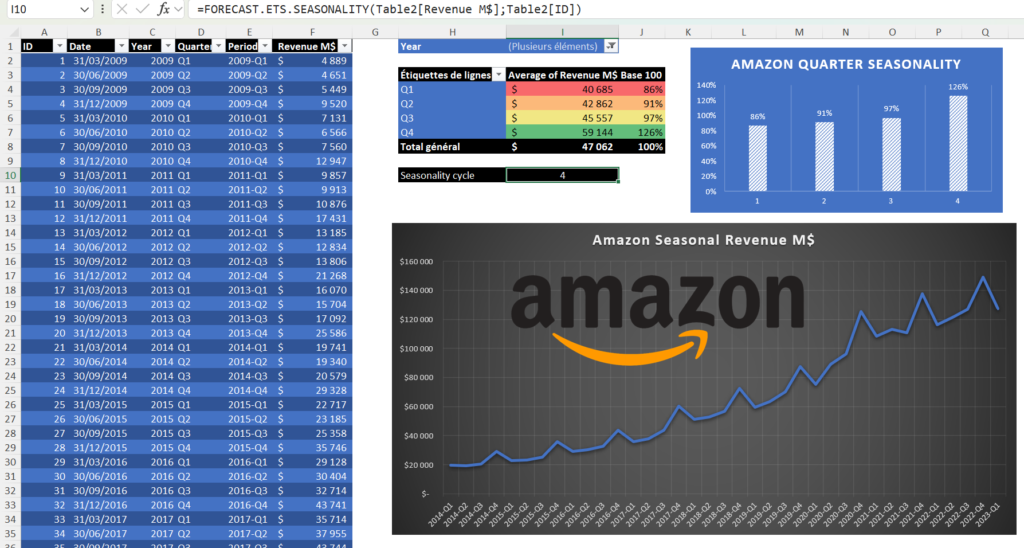
The formula indicates 4. This means a new cycle every 4 periods. Given that we have quarterly data, this is an annual cycle.

This approach is particularly useful if you are unsure of the seasonality present in your data.

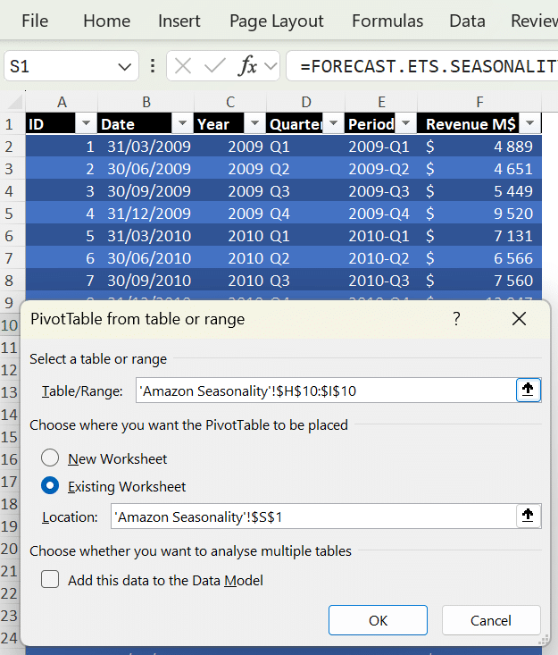
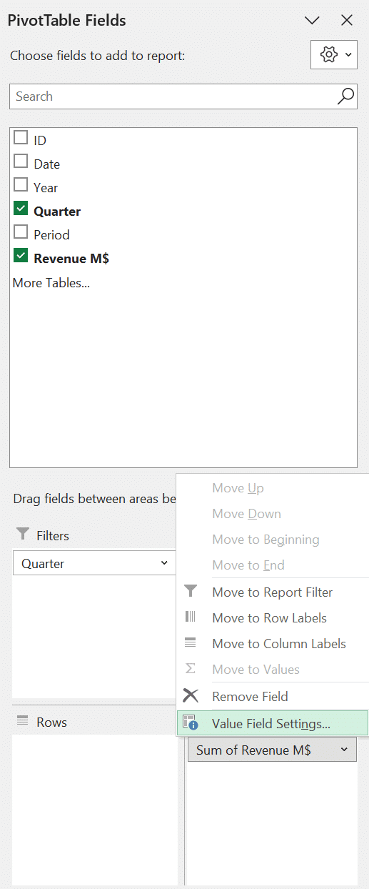
For the rest of this example, we’ll calculate the average weight of each quarter as a percentage, which we’ll then use to derive a sales forecast. For that purpose, we’re going to use a pivot table:

• Click on insert: pivot table
• Select: Existing worksheet and position yourself in S1, for example.
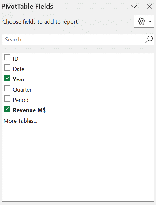
• Tick: Quarter and Revenue M$

This gives the total income for each quarter.

However, we want to calculate the average income.

All you need to do is :

• Select Quarter and bring it in the filter field
• Put Revenue M$ in the Value field
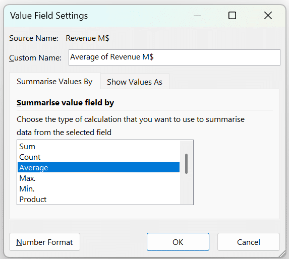
• Click on Value Field Setting to display the average instead of the sum.

Based on these results, we will determine the weight of each quarter.

Let’s position ourselves in an empty cell:

• Divide the reference of the Pivot Table cell corresponding to the average of Q1 by that of the total sum, locking it with the $ (in my case = T4/$T8)
• Convert the result to a % format
• Drag the formula down

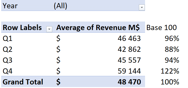
Here, we find what I call a base 100, which can also be called a seasonality coefficient or normalization in relation to the annual average.

Values are expressed in relation to a common base (the annual average = 100%).

It’s clear that the fourth quarter (Q4) consistently carries more weight than the second quarter (Q2), which is typically quieter, averaging an 88% weighting.

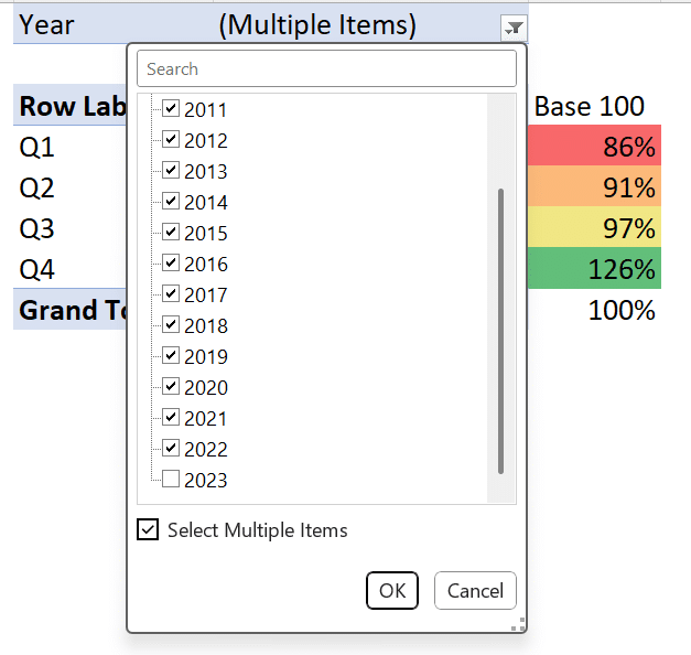
These averages are calculated from 2009 to 2023. To be more precise, we can remove the current year (here, 2023) because it is not complete and therefore biases the data very slightly.

In that purpose, we will filter and uncheck 2023 :

Calculation of quarterly sales forecasts

Based on these elements, we can draw up a sales forecast. Let’s go back to our example and perform the following operation:

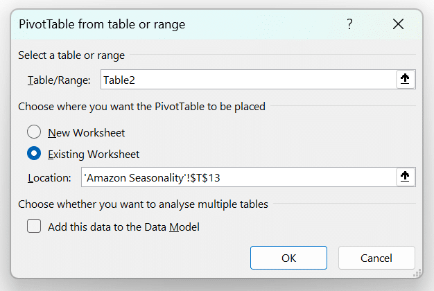
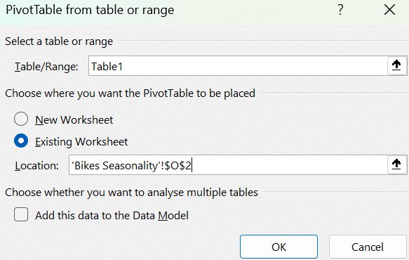
• Insert > Pivot Table from Table / Range
• We can insert it in T13, for example

• This time we select the years, and the sum of income

This brings us back to Amazon’s billion-dollar turnover.

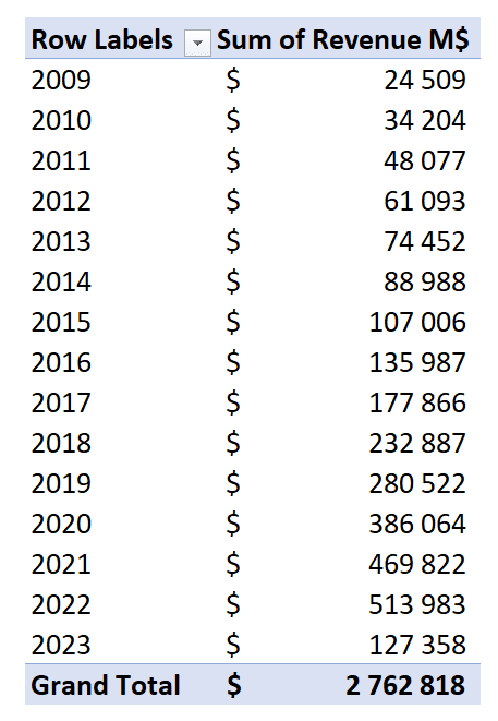
The previous year (2022) revenues were $513 billion.

Now imagine that Amazon’s CEO announces a revenue target of $600 billion for the following year. The question then becomes: how should this forecast be broken down by quarter?

We can proceed as follows:

• In W13, for example, let’s write 2023
• In X13, we note: 600,000 according to Amazon’s CEO.
• from W14 to W17 insert Q1, Q2, Q3 and Q4
• In X14, we will write: ” = $X$13*V5″ (the annual target multiplied by the base 100 coefficient), and we will spread the formula
• Then format in dollars

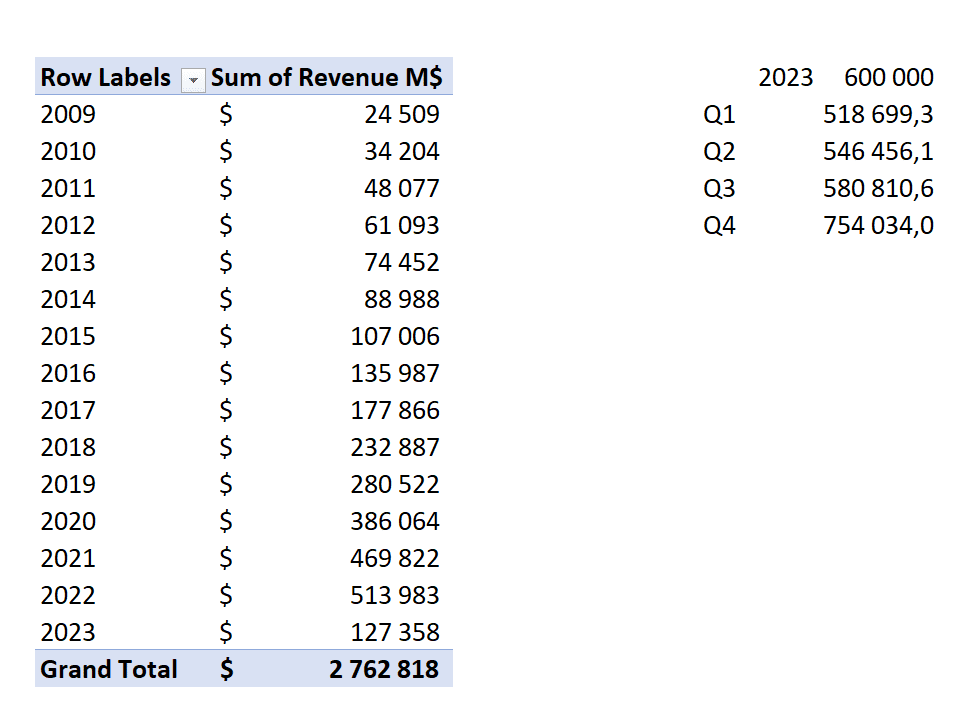
Then we’ll go back to cell X14 and divide it by 4 (to convert an annual target into a quarterly one): =$X$13*V5/4

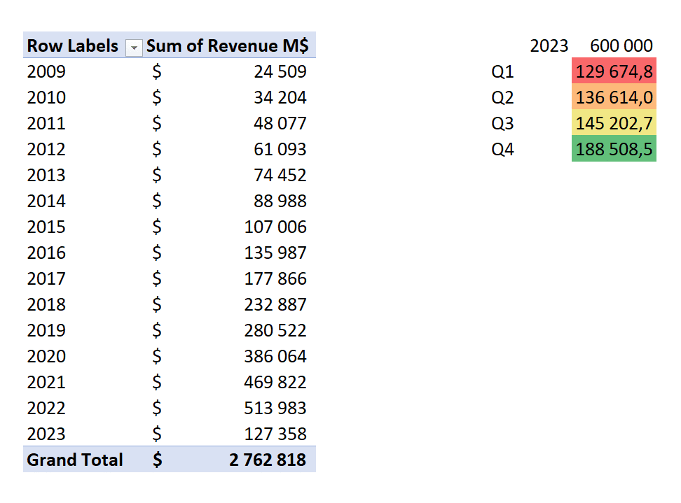
Revenue is forecasted at $129 billion for the first quarter, down from $188 billion in the previous quarter. This reflects the seasonal distribution of sales, with a stronger concentration toward the end of the year.

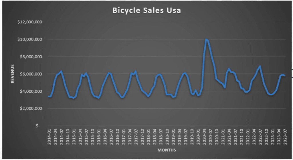
Bicycle sales in the USA example

Calculating sales forecasts by month

We are now applying the same principle to a monthly analysis.

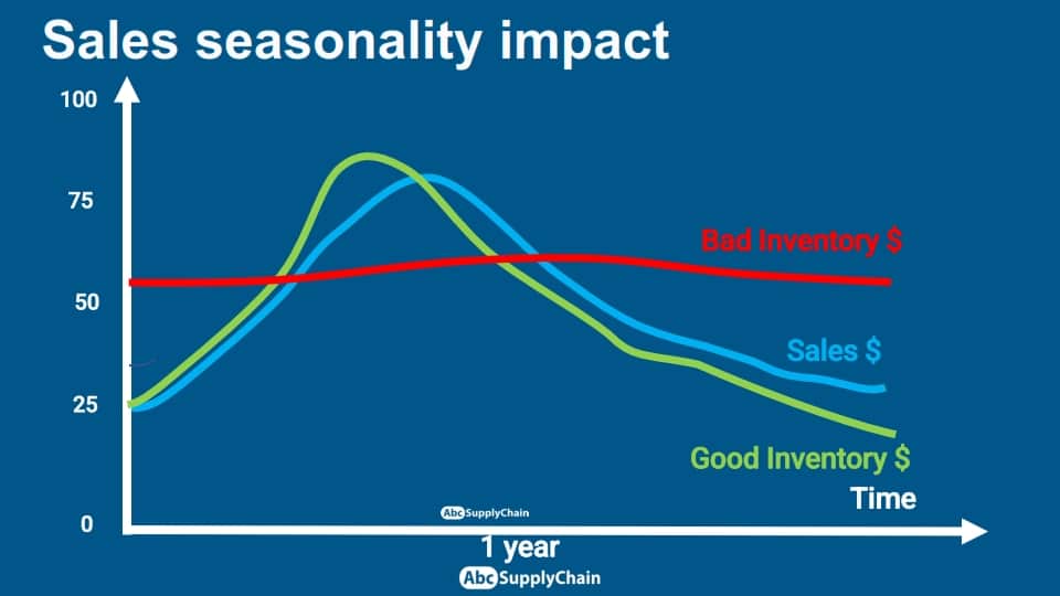
Let’s take the example of bicycle sales in the United States: there was an exceptional peak during the pandemic, commonly referred to as an “outlier.”
This peak significantly disrupted the supply chain, causing both stockouts and overstock situations. In this exercise, the objective is to rebuild a base 100 to better understand seasonality by neutralizing this exceptional event.

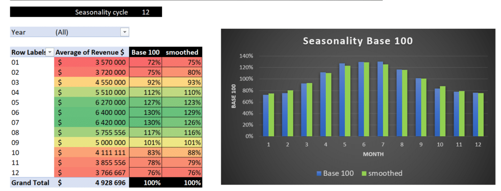
To do this, we’re going to create a new pivot table in the second tab :

• Insert > Pivot table from a table or range
• This time we’re filtering by month
• In the value field setting, let’s indicate average.

Once the table has been inserted, you can refine the table:

• We format revenues in dollars as we did previously
•  Integrate the base 100 calculation by dividing the first value by the grand total, using the formula =P4/$P$16.
• Spread the formula
• Format as a percentage

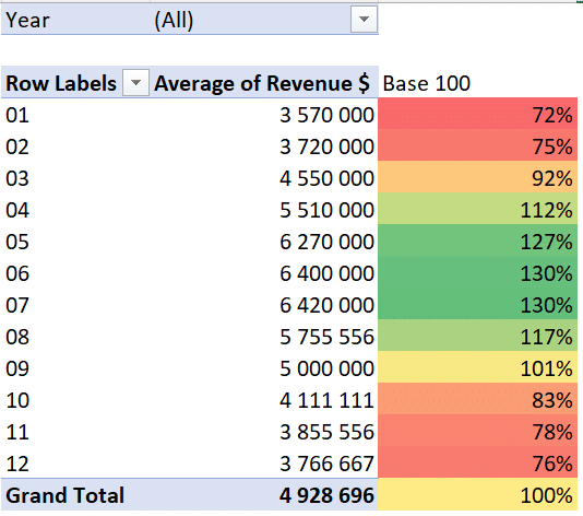
There is a fairly marked peak in 2020, the pandemic period. We can deselect 2020 in the filter. The principle is to deliberately exclude an atypical year in which the data was particularly disrupted. Once this has been done, we find a trend that is much more cyclical and consistent with the market’s usual behaviour.

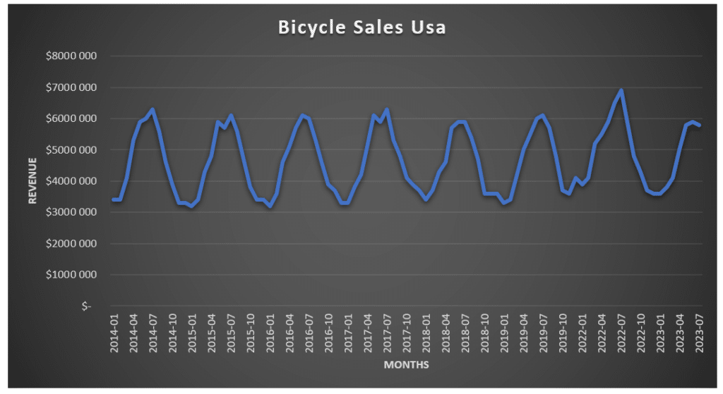
By recreating the formula, we can clearly observe a recurring 12-month cycle—an annual pattern—with a peak in sales during the spring, similar to what we typically see with products like tents.

It’s essential to analyse these trends graphically and with figures, especially when behaviour is out of the ordinary. In this particular case, I have deliberately excluded an atypical year to obtain a more representative seasonal base. From this base, you can then break down your annual forecasts month by month, enabling you to better anticipate sales, purchases, budgets, and financial requirements.

Bonus: automatic data smoothing

Here is a useful tip: When you don’t have much data or when sales are very irregular, it becomes difficult to identify a clear trend. This is where automatic data smoothing comes in, one of several methods I use regularly. It makes time series more readable and usable.

This technique, with detailed formulas, is provided in the Excel file provided. In the example shown here, the volumes are large enough for there to be little variation, but in other contexts, this cleaning can make all the difference.

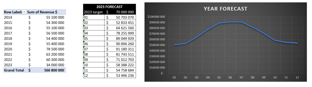
You will also see how to derive the annual forecast based on a $70M target for 2023.

Aggregation and accuracy of sales forecasts

How do you determine the level of aggregation (granularity)?

Determining the right level of aggregation to analyse seasonality is an essential—and sometimes complex—step. I often spend hours, even days, discussing this question with the professionals I work with in my school.

In practice, seasonality can be analyzed at various levels:

• Geographical: by warehouse, by region, by country, or even globally.
• Product-based: by reference, by family, by category, by brand, or at total portfolio level.
• Temporal: yearly, quarterly, monthly, weekly or even daily.

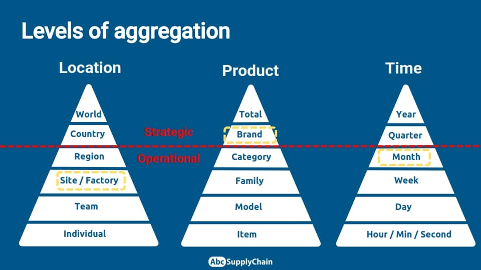
With this example, we are working at a fairly standard level: by site, by brand, and by month. At this level, we can already see trends clearly and structure a relevant seasonal pattern.

The right level will always depend on the purpose of your forecast. Is it to plan local sourcing? To guide global purchasing? To manage weekly marketing campaigns? Before you start, always ask yourself: What is this forecast going to be used for? What level of operational or strategic need do you need to address?

Once you have clarified this intention, a more in-depth analysis will enable you to identify a clear, recurring seasonal cycle for the granularity chosen.

Warning: beyond the method, the quality of the data is essential. We need to ensure that the categories selected are consistent, well-defined and, above all, homogeneous. Otherwise, there is a risk that the seasonality generated will be distorted or of little use.

Therefore, a thorough cleaning up and structuring of the data upstream is essential if we are to draw reliable, actionable conclusions.

How can we improve the reliability of our forecasts?

The starting point is a clear understanding of your objectives. Why are you introducing seasonality? What specific purpose should it serve in your forecasts?

Many companies I work with have poor forecast accuracy. And that’s not surprising: the environment is uncertain, the data is sometimes incomplete, and the processes are not clear, structured, or automated.

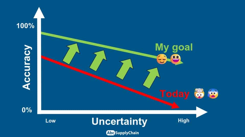
That’s why rigorous work on seasonality is essential: not only does it improve forecasts, but it also builds a more solid foundation for all decision-making.

Become a Forecasting Expert: My Method

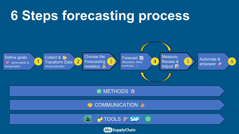
I’ve put in place a complete six-step forecasting method. This approach is not limited to technical aspects, it also covers the entire process: from defining objectives to effective communication, including the use of the right tools and methods.

The aim is to empower your teams so that you can concentrate on what really adds value to your business.

Frequently Asked Questions About Forecast Seasonality